OpenCV: Epipolar Geometry
Goal In this section, We will learn about the basics of multiview geometry We will see what is epipole, epipolar lines, epipolar constraint etc. Basic Concepts When we take an image using pin-hole camera, we loose an important information, ie depth of the
docs.opencv.org
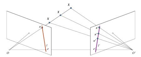
그림에서 보다 시피 단안만을 이용하면 X의 투영되는 점이 OX 선중 어떤 3D 상의 점인지 알기 어렵다. 하지만, 다른 각도의 이미지를 활용하면 OX 선분 상의 점이 오른쪽 이미지의 다른 위치에 투영된다. 따라서 두 이미지를 활용하여 3D 지점을 삼각 측량(Triangulation)을 이용해서 구할 수 있다.
점 x가 놓일 수 있는 다른 이미지 상의 선분을 Epiline이라 한다 (오른쪽 이미지 전체에서 검색하지 않아도 된다)
왼쪽 이미지 상의 모든 점 x가 오른쪽 이미지 상의 선분과 대응되며 이러한 관계를 Epipolar Constraint 라고 한다.
XOO'를 Epipolar Plane 이라 한다.
import numpy as np
import cv2 as cv
from matplotlib import pyplot as plt
img1 = cv.imread('myleft.jpg',0)  #queryimage # left image
img2 = cv.imread('myright.jpg',0) #trainimage # right image

# -------------------------------------------------------------- #
# 1) find_matching_keypoints
sift = cv.SIFT_create()

# find the keypoints and descriptors with SIFT
kp1, des1 = sift.detectAndCompute(img1,None)
kp2, des2 = sift.detectAndCompute(img2,None)

# FLANN parameters
FLANN_INDEX_KDTREE = 1
index_params = dict(algorithm = FLANN_INDEX_KDTREE, trees = 5)
search_params = dict(checks=50)
flann = cv.FlannBasedMatcher(index_params,search_params)
matches = flann.knnMatch(des1,des2,k=2)
pts1 = []
pts2 = []
# ratio test as per Lowes paper
for i,(m,n) in enumerate(matches):
    if m.distance < 0.8*n.distance:
        pts2.append(kp2[m.trainIdx].pt)
        pts1.append(kp1[m.queryIdx].pt)

# -------------------------------------------------------------- #
# 2) find Fundamental Matrix
pts1 = np.int32(pts1)
pts2 = np.int32(pts2)
F, mask = cv.findFundamentalMat(pts1,pts2,cv.FM_LMEDS)

# We select only inlier points
#pts1 = pts1[mask.ravel()==1]
#pts2 = pts2[mask.ravel()==1]

# -------------------------------------------------------------- #
# 3) Find epilines corresponding to points in right image (second image) and
# drawing its lines on left image
# pts2와 F로 부터 대응되는 epilines를 구한다.
# ★ pts 포맷 : (n, 1, 2) / ★ lines 포맷 : (n, 1, 3)
lines1 = cv.computeCorrespondEpilines(pts2.reshape(-1,1,2), 2,F)
lines1 = lines1.reshape(-1,3) # (n, 1, 3) -> (n, 3)
# ★ img1에다가 lines1을 그린다. img1, img2에 점은 공통으로 그린다.
img5,img6 = drawlines(img1,img2,lines1,pts1,pts2)

# Find epilines corresponding to points in left image (first image) and
# drawing its lines on right image
lines2 = cv.computeCorrespondEpilines(pts1.reshape(-1,1,2), 1,F)
lines2 = lines2.reshape(-1,3)
img3,img4 = drawlines(img2,img1,lines2,pts2,pts1)
plt.subplot(121),plt.imshow(img5)
plt.subplot(122),plt.imshow(img3)
plt.show()
여기서 line은 (n, 3)을 가지는데 한 열당 가지는 값인 (a, b, c)는 아래 선분을 의미한다.
$$ ax + by + c = 0 $$
https://docs.opencv.org/4.x/d9/d0c/group__calib3d.html#ga19e3401c94c44b47c229be6e51d158b7

'심화 > 영상 - 구현 및 OpenCV' 카테고리의 다른 글
| OpenCV는 Row-Major, Matlab은 Column-Major (0) | 2022.11.14 |
|---|---|
| erode & dilate (2) | 2022.10.29 |
| ORB (Oriented FAST and Rotated BRIEF) (0) | 2022.03.15 |
| Optical Flow (0) | 2021.06.21 |
| Fast Algorithm for Corner Detection (0) | 2021.06.19 |


